Dynamic Programming

Introduction

Dynamic Programming is a mathematical tool for finding the optimal algorithm of a problem, often employed in the realms of computer science.

During the autumn of 1950, Richard Bellman, a tenured professor from Stanford University began working for RAND (Research and Development) Corp, whom suggested he begin work on multistage decision processes. During the 1950s, Charles Erwin Wilson was the Secretary of Defence for the United States, and as RAND was employed by the U.S Air Force, Wilson was virtually their boss. Wilson, originally an electrical engineer, ironically had a hatred for the word ‘research’, and so Bellman had to come up with an alternative name to hide the fact that he was purely researching mathematics. To convey that Bellman’s research was about planning and decision making, he used the word ‘programming’, and prefixed it with ‘dynamic’, to convey that it was multistage and had time variances [1]. Bellman, due to the aforementioned recommendations by RAND, developed an approach that would break down a large or complex problem into a series of smaller problems. Through solving these smaller problems, the optimal solution to the overall problem is discovered.

The aim of Dynamic Programming is the use of past values for the procurement of a solution to a problem. This is done to avoid unnecessary computation of the same calculation that problems may contain, optimising, enabling computer algorithms to run as efficiently as possible. It aims to find the optimal substructure of a problem (if it exists), and to eliminate any occurrences of overlapping sub problems.

Dynamic Programming works in contrast to Linear Programming. Whilst it is concerned with functional relations and multi-stage decision processes, Linear Programming is a method used to achieve the best result based upon linear relationships [2].

Optimal Substructures

When Dynamic Programming is applied, breaking up a problem and reconstructing it, we often find the optimal substructure of a problem. A solution is said to have an optimal substructure if it can be defined based upon optimal solutions of its sub problems.

For example, the shortest path problem has the optimal substructure property. If we have three sequentially placed locations, X, Y, and Z, and we wish to find the optimal distance of X to Z. The solution can be defined as the sum of the optimal solutions between X to Y, and Y to Z, therefore X to Z can be defined based upon the optimal solutions of it’s sub problems.

Overlapping Sub-Problems

A problem or function contains overlapping problems if it can be broken down into a series of smaller problems, and some are duplicates. The need for the problem to compute the same calculation many times over can cause large increases in the running time of the problem. Dynamic Programming aims to remove the need to compute the same calculations multiple times.

Memoisation

Memoisation , also known as caching, is a technique used in Computer Science, which stores the results of functions and calculations, and uses them if the calculations are needed again. Due to the fact that memory is finite, memoisation is not feasible in all situations, and thus, needs to be used appropriately and sparingly, especially when it comes to large applications. Tail recursion [3], a variant of traditional recursion implements memoisation, which uses memoisation very economically.

Fibonacci: An elementary use of Dynamic Programming

One of the simplest problems that can be optimised with a Dynamic Programming approach is the Fibonacci number. The Fibonacci number (also known as the Fibonacci sequence) is a series of numbers where the leading number is the sum of the previous two numbers (modern interpretation) [4].

0,1,1,2,3,5,8,13,21,34…

It is named after Italian mathematician Leonardo of Pisa (commonly known as Fibonacci), whom described the sequence in his book Liber Abaci during 1202 AD. It had previously been described in Indian Mathematics, but had not yet encountered the western world [5].

Fibonacci can be described as follows;

F0 = 0
F1 = 1
Fn = F(n-1) + F(n-2),

For example;

F3 = F(2)  + F(1)
F3 = (F(1) + F(0))  + 1
F3 = (1 + 0) + 1
F3 = 2

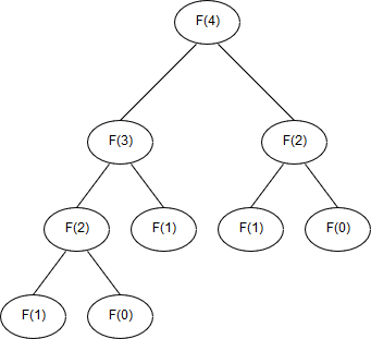
This poses a problem. Computing a Fibonacci number greater than two will force overlapping sub problems.

The figure above represents the structure of the Fibonacci sequence of four. The Fibonacci number of four will compute the Fibonacci of two twice. The number of overlapping sub problems will grow exponentially as the Fibonacci number is increased, and thus the running time to compute it.

We can use Dynamic Programming (and memoisation) to mitigate these unneeded computations, and define the Fibonacci Number of n as follows;

Fibonacci (n, i = 0, a = 0, b = 1 )
{
      if ( i < n )
        Fibonacci( n, i+1, b, a+b )
      return b;
}

This approach first checks if we have reached the desired number, if not, it computes the sequence. It will never call a number that has already been calculated, and will instead use memoisation and pass the previous (to the current number we are at) two values to the function to calculate them.

Economic Optimisation: A Canonical example of dynamic programming.

Various economic problems, especially around stage based decision making can be solved through the use of dynamic programming.

Michael Trick describes the following problem. A corporation owning a number of plants has funds to invest, with each of the plants providing a number of proposals of what returns it can provide depending on how many funds it is allocated. This problem can be solved quite nicely with dynamic programming [6].

The total number of solutions is the number of proposals in each plant multiplied, in Ticks case there are 24 possible solutions (3 x 4 x 2). Enumerating of all solutions is infeasible due to the fact that many solutions may not be possible with the funds available, and are not worth calculation, and for problems containing lots of proposals, it may not be computationally feasible. Enumerating over all solutions is also not efficient, we do not look at previous solutions to eliminate possible, inferior (less generated revenue) solutions.

This is where dynamic programming can come into use. We can employ it to develop a solution that will take into consideration the available funds as well as previously tested solutions.

Solution Design

A solution was developed using dynamic programming to approach this problem, written in C++.

Proposals

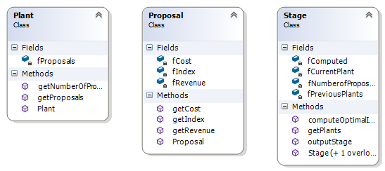
Proposals contain three integers, an index (their position in the plant), as well as their cost, and revenue. These are only set in the constructor and can be accessed but not changed.

Plant

Each plant contains a vector of proposals, which it creates when the constructor is invoked. It can return a reference to the vector of it’s proposals, as well as the number of proposals it contains.

Stage

This class contains the algorithm. Each state maintains a list of proposals (from the given plant), as well as a map, it’s key the cost, and value the revenue it generates. The stage takes a previous stage (or null if it is the first).

If it is the first stage, then revenue is just the possible proposals that cost less than the funds available. If we are on any of the stages after the initial, we begin iterating through each of the proposals. If the cost of that proposal is less than or equal to the available funds, then we assign the revenue to a temporary variable, and if any funds remain, we access the revenue from the previous stage for the remaining funds, adding it to the temporary variable. It is then checked against the previous stage’s revenue for that cost. If it is greater, then it is the new revenue for that cost, if not, we get use the previous stage’s revenue for that cost.

This solution uses Tail Recursion. Each stage does its necessary calculations, then passes its information to the next stage which is the natural solution to the problem. Each stage will asses it’s plant’s proposals compared to the available funds, and then pass its information to the next stage. Whilst the approach finds the best solution, it does not return the proposals used, only the possible revenue and the cost it will require. The map of cost to revenue, implements the memoisation aspect of the algorithm.

if first stage
  foreach proposal in plant
    if proposal cost <= available funds
      if Revenue[proposal cost] < revenue of new proposal
        Revenue[proposal cost] = revenue of new proposal
else
  foreach proposal in plant
    if proposal cost <= available funds
      revenue = proposal revenue
      remaining funds = funds - proposal cost
      if remaining funds > 0
        (revenue-1,cost-1) = max Stage-1[remaining funds]
      revenue += revenue-1
      cost = propsal cost + cost-1
      if Revenue[cost] < revenue
        Revenue[cost] = revenue

Whilst solvable, Trick makes several assumptions. Firstly, his solution assumes that each plant will have a proposal enacted upon, and secondly, that we use all the funds with the remainder not included in the revenue created in the end.

Conclusion

Dynamic Programming is an essential tool for solving multistage problems. It helps find the optimal substructure of a problem where possible, and remove any overlapping sub problems. It is applicable for smaller problems, such as Fibonacci, and larger problems such as economic optimisations. This report is by no means an extensive or advanced approach to dynamic programming, and aims only to introduce the concept of dynamic programming, and explain how it works on a rudimentary example.

References

• [1] R. Bellman, Eye of the hurricane. Singapore: World Scientific, 1984
• [2] S. Dreyfus, “A Comparison of Linear Programming and Dynamic Programming”, RAND, 1956.
• [3] D. Friedman and M. Want, Essentials of Programming Languages. MIT Press, 1999.
• [4] “Fibonacci number”, En.wikipedia.org, 2017. [Online]. Available: https://en.wikipedia.org/wiki/Fibonacci_number. [Accessed: 22- Oct- 2017].
• [5] L. Fibonacci and L. Sigler, Fibonacci’s Liber abaci. New York: Springer, 2003.
• [6] M. Trick, “A Tutorial on Dynamic Programming”, Mat.gsia.cmu.edu, 2017. [Online]. Available: http://mat.gsia.cmu.edu/classes/dynamic/dynamic.html. [Accessed: 30- Oct- 2015].
  
  

The source code can be found here.